SimPLE: Similar Pseudo Label Exploitation for Semi-Supervised Classification

Introduction

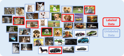
Deep learning has recently achieved state-of-the-art performance on many computer vision tasks. labeling large datasets is very expensive and often not feasible, especially in domains that require expertise to provide labels. Semi-Supervised Learning (SSL), on the other hand, can take advantage of partially labeled data, which is much more easily available, as shown in Figure 1, for example.

Semi-supervised Learning

A critical problem in semi-supervised learning is how to generalize the information learned from limited label data to unlabeled data. Following the continuity assumption that close data have a higher probability of sharing the same label, many approaches have been developed, including the recently proposed Label Propagation.

Another critical problem in semi-supervised learning is how to directly learn from the large amount of unlabeled data. Maintaining consistency between differently augmented unlabeled data has been recently studied and proved to be an effective way to learn from unlabeled data in both self-supervised learning.

The recently proposed MixMatch combines the above techniques and designed a unified loss term to let the model learn from differently augmented labeled and unlabeled data, together with the mix-up technique, which encourages convex behavior between samples to increase model’s generalization ability. ReMixMatch further improves the MixMatch by introducing the distribution alignment and Augmentation Anchoring techniques, which allows the model to accommodate and leverage from the heavily augmented samples. FixMatch simplified its previous works by introducing a confidence threshold into its unsupervised objective function and achieves state-of-the-art performance over the standard benchmarks.

In this paper, we propose to take advantage of the relationship between different unlabeled samples. We introduce a novel Pair Loss, which encourages a pair of similar unlabeled samples (in the augmented space) to have similar predictions if at least one of them is of high confidence in its prediction. Combining the techniques developed by the MixMatch family, we propose the SimPLE algorithm. As shown in Figure 2, the SimPLE algorithm generates pseudo labels of unlabeled samples by averaging and sharpening the predictions on multiple weakly augmented variations of the same sample.

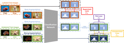
Then, we use both the labels and pseudo labels to compute the supervised cross-entropy loss and unsupervised $L2$ distance loss. These two terms push the decision boundaries to go through low-density areas and encourage consistency among different variations of the same samples. Finally, with the newly proposed Pair Loss, we harness the relationships among the pseudo labels of different samples by encouraging consistency among different unlabeled samples which share a great similarity.

Method

To take full advantage of the vast quantity of unlabeled samples in SSL problems, we propose the SimPLE algorithm that focuses on the relationship between unlabeled samples.

Problem Description

We define the semi-supervised image classification problem as following. In a $L$-class classification setting, we have:

• $\mathcal{X}=\left(\left(x_{b}, y_{b}\right) ; b \in(1, \ldots, B)\right)$: a batch of labeled data
• $\mathcal{U}=\left(u_{b} ; b \in(1, \ldots, B)\right)$: a batch of unlabeled data
• $\mathrm{p}_{\text{model}}\left(\tilde{y} \mid x ; \theta\right)$: the model’s predicted softmax class probability of input $x$ parameterized by weight $\theta$

Augmentation Strategy

Our algorithm uses Augmentation Anchoring, in which pseudo labels come from weakly augmented samples act as “anchor,” and we align the strongly augmented samples to the “anchor.” Our weak augmentation, follows that of MixMatch family, contains a random cropping followed by a random horizontal flip. We use RandAugment or a fixed augmentation strategy that contains difficult transformations such as random affine and color jitter as strong augmentation. For every batch, RandAugment randomly selects a fixed number of augmentations from a predefined pool; the intensity of each transformation is determined by a magnitude parameter.

Pseudo-labeling

Our pseudo labeling is based on the label guessing technique used in MixMatch. We first take the average of the model’s predictions of several weakly augmented versions of the same unlabeled sample as its pseudo label. As the prediction is averaged from $K$ slight perturbations of the same input instead of $K$ severe perturbation or a single perturbation, the guessed pseudo label should be more stable. Then, we use the sharpening operation defined in MixMatch to increase the temperature of the label’s distribution: $$\operatorname{Sharpen}(p, T):= \frac{p^{\frac{1}{T}}}{\textbf{1}^\top p^{\frac{1}{T}}}$$

As the peak of the pseudo label’s distribution is “sharpened,” the network will push this sample further away from the decision boundary. Additionally, following the practice of MixMatch, we use the exponential moving average of the model at each time step to guess the labels.

Loss

Our loss consists of three terms, $\mathcal{L_X}$, $\mathcal{L_U}$, and $\mathcal{L_P}$, representing the supervised loss, the unsupervised loss, and the Pair Loss respectively.

$$ \begin{align} \mathcal{L} &= \mathcal{L_X} + \lambda_{\mathcal{U}} \mathcal{L_U} + \lambda_{\mathcal{P}} \mathcal{L_P} \\
\mathcal{L_X} &= \frac{1}{\left| \mathcal{X}' \right|} \sum_{x,y \in \hat{\mathcal{X}}} H\left(y, \mathrm{p}_{\text{model}}\left(\tilde{y} \mid x ; \theta\right)\right) \\
\mathcal{L_U} &= \frac{ \sum_{u,q \in \hat{\mathcal{U}}} \mathbb{1}_{\left(\max\left(q\right) > \tau_c\right)} \left| q - \mathrm{p}_{\text{model}}\left(\tilde{y} \mid u ; \theta\right) \right|^{2}_{2} }{L \left| \hat{\mathcal{U}} \right|} \end{align} $$

$\mathcal{L_X}$ calculates the cross-entropy of weakly augmented labeled samples, and $\mathcal{L_U}$ represents the $L_2$ distance between strongly augmented samples and their pseudo labels, filtered by high confidence threshold. Notice that $\mathcal{L_U}$ only enforces the consistency among different perturbations of the same samples but not the consistency among different samples.

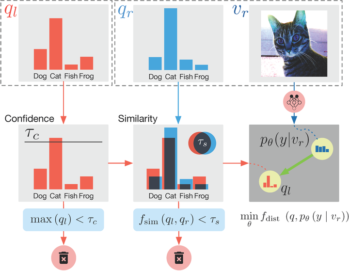
As we aim to exploit the relationship among unlabeled samples, we hereby introduce a novel loss term, Pair Loss, that allows information to propagate implicitly between different unlabeled samples. In Pair Loss, we use a high confidence pseudo label of an unlabeled point, $p$, as an “anchor.” All unlabeled samples whose pseudo labels are similar enough to $p$ need to align their predictions under severe perturbation to the “anchor.”

Figure 3 offers an overview of this selection process. During this process, the similarity threshold “extended” our confidence threshold in an adaptive manner, as a sample whose pseudo label confidence is below the threshold can still be selected by the loss and be pushed to a higher confidence level. Formally, we defined the Pair Loss as following:

$$ \begin{aligned} \mathcal{L_P} &= \frac{1}{\binom{K’B}{2}} \sum_{ \substack{ i,j \in \left[\left|\mathcal{U}'\right|\right], i \ne j \\
\left(v_l, q_l\right) = \mathcal{U}'_{i} \\
\left(v_r, q_r\right) = \mathcal{U}'_{j} } } \varphi_{\tau_c}\left(\max\left(q_l\right)\right) \\
&\cdot \varphi_{\tau_s}\left(f_{\operatorname{sim}}\left(q_l, q_r\right)\right) \\
&\cdot f_{\operatorname{dist}}\left(q_l, \mathrm{p}_{\text{model}}\left(\tilde{y} \mid v_r ; \theta\right)\right) \end{aligned} $$

Here, $\tau_c$ and $\tau_s$ denote the confidence threshold and similarity threshold respectively. $\varphi_t(x)=\mathbb{1}_{\left(x > t\right)} x$ is a hard threshold function controlled by threshold $t$. $f_{\operatorname{sim}}\left(p, q\right)$ measures the similarity between two probability vectors $p, q$ by Bhattacharyya coefficient. The coefficient is bounded between $[0, 1]$, and represents the size of the overlapping portion of the two discrete distributions:

$$f_{\operatorname{sim}}\left(p, q\right) = \sqrt{p} \cdot \sqrt{q}$$

$f_{\operatorname{dist}}\left(p, q\right)$ measures the distance between two probability vectors $p, q$. As $f_{\operatorname{sim}}\left(p, q\right)$ is bounded between $[0, 1]$, we simply choose the distance function to be $f_{\operatorname{dist}}\left(p, q\right) = 1 - f_{\operatorname{sim}}\left(p, q\right)$.

Although based on analysis, we found that $\cos(\cos^{-1}(\sqrt{\tau_c})+\cos^{-1}(\tau_s))^2$ is the minimal confidence a label need to have for it to be selected by both thresholds, such low confidence label are rarely selected in practice. Based on empirical evidence, we believe this is caused by the fact a label $p$ that can pass through the high confidence threshold typically has a near one hot distribution. Thus, for another label $q$ to fall in the similarity threshold of $q$, it must also have relatively high confidence. Due to this property, the Pair Loss is not very sensitive to the choices of hyperparameters $\tau_s$, $\tau_c$, which we will show empirically in later section.

SimPLE Algorithm

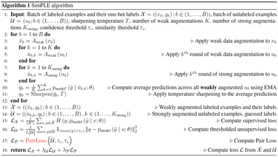
By putting together all the components introduced in this section, we now present the SimPLE algorithm. During training, for a mini-batch of samples, SimPLE will first augment both labeled and unlabeled samples with both weak and strong augmentations. The pseudo labels of the unlabeled samples are obtained by averaging and then sharpening the models' predictions on the weakly augmented unlabeled samples. Finally, we optimize the three loss terms based on augmented samples and pseudo labels. During testing, SimPLE uses the exponential moving average of the weights of the model to do prediction, as what is done by MixMatch. Figure 2 gives an overview of the algorithm, and the complete training algorithm is described in Alg. 1.

The experiment section will be updated soon